
Segger documentation: Aligning structures to regions
- GroEL
- Bacteriophage lambda
1.1 Segmenting the map
First, the density map must be segmented. Here we will use as an example the density map of GroEL at 4.2Å resolution. This map can be download from this link. When this map is segmented (as described on the segmentation page) at a threshold of 0.89, and the regions are grouped using 4 steps of size 7.5Å, 14 regions are obtained, with each region corresponding to a single protein. The density map and segmented regions are shown below.
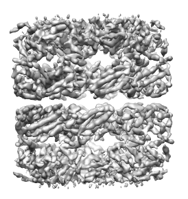
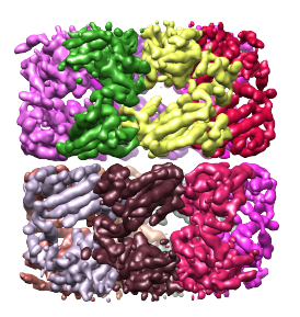
Side note: the segmentation threshold does not actually influence the number of regions obtained. At other thresholds (at which the background noise is not included), the same number of regions can be obtained by the smoothing and grouping method.
Side note: For this example we used large smoothing steps intentionally. When taking smaller steps, less accurate segmentation regions were obtained. This may be attributed to noise in the density map. Applying more smoothing in the first step is helping to suppress this noise.
1.2 Obtaining the structure of a single protein
The structure of a single protein in GroEL can be obtained from PDB:1xck. After downloading this structure, it should be placed in the same directory as the segmented GroEL density map (emd_5001.mrc). It can then be opened using the Segger interface, by clicking on the drop-down menu to the right of the Structure button. This drop-down menu shows all PDB files in the same dirctory as the selected density map (which should be emd_5001.mrc). Selecting 1XCK.pdb will open the structure.
Select a single chain of this structure, e.g. chain A, and save it to its own PDB file, e.g. 1xck_A.pdb. Then use the drop-down menu to select and open this structure by itself. Alternatively, you can delete all chains other than A, and then choose 1xck.pdb in the drop-down menu.
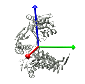
Once the structure of a single protein is selected in the drop-down menu to the right of the Structure button, first click the Center button to position this structure such that its center is at the origin, and its principal axes point along the X, Y, and Z axes. The principal axes can be shown by selecting Structure->Show Axes. The structure and axes are shown in the image below.
1.3 Generating a density map of the structure
A density map must be simulated for the structure, to allow the computation of a cross-correlation score, and cross-correlation based local refinement. The density map should be simulated using roughly the same resolution and grid spacing as the cryo-EM density map. For the GroEL density map used here, enter 4.2,1.06 in the field to the right of "map resolution, step size:". Then, to simulate the map, click the Generate density button.
The density map will appear in the main Chimera window. Its name, 1xck_A_r4.2_sp1.1.mrc, will also appear in the drop-down menu to the right of the Structure density map button. This map can be manipulated like any other density map in the "Volume Viewer" interface. It can be hidden either through the Model Panel or Volume Viewer dialogs, so as to allow the structure to be seen; whether it is shown or hidden does not influence the steps to follow.
1.4 Aligning the structure to a single region
We can now align this structure to a segmented region in the density map. One way to do this is using the principal-axes transform. To see how this would work, select a single segmented region, and then select Regions->Show only selected, to show this region alone, then Regions->Make transparent to allow us to see through the region surface, and then Regions->Show axes for selected to show the principal axes for this region. The resulting view is shown in the image below.
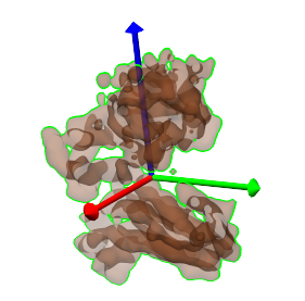
By looking at the two images above, shown again below side by side, it can be seen that principal axes are roughly the same with respect to the structure and to the region. The structure can thus be aligned to the region by matching the centers and the principal axes of the structure to those of the region.


To perform the alignment, simply select Align to->Selected region in the Segger interface (make sure the region is still selected). Because the sign of the principal axes are ambiguous, 4 possible alignments are tried, and the one that gives the highest cross-correlation is kept. Each alignment is locally refined (using the Chimera 'fit-in-map' procedure'), locally maximizing the cross-correlation score starting with each alignment. The latter is critical in picking the correct alignment, because after local optimization, the cross correlation scores of correct alignments are typically much higher (x2 or more) than cross-correlations scores of non-correct alignments. The resulting alignment is shown below. The structure, shown as a ribbon, can be seen to match the segmented region, shown using the transparent surface, quite well.
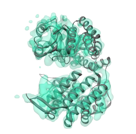
Because the alignment is direct, this process is extremely fast and takes only a few seconds. By comparison, exhaustive search looks through all possible positions and orientations of the structure in the density map, which can take on the order of minutes. However, the principal axes alignment may not always work, especially for structures that are spherical, for example. In such cases, a more direct alignment rather than exhaustive search is still possible. The alignment involves matching the centers, and then searching only through different orientations. This alignment mode can be selected instead of the principal axes alignment by selecting Align to->By rotation in the Segger interface. In this example, doing the alignment this way will produce the same result. Though it will take a bit longer, it's still faster than exhaustive search.
Side note: Showing the principal axes of the structure or the region is not required to complete the alignment process. They are only shown here for illustrative purposes.
Important side note: When aligning a structure to a region, make sure that the non-smoothed density map is selected in the field to the right of "Density map" (in this example: emd_5001.mrc) , and the regions file in which the selected region resides is selected in the field to the right of Regions (#), where # is the number of regions in the file. The selected density map is very important in the alignment process - it provides the density values against which the density values in the simulated map of the structure are compared against, and which are used to optimize the fit. The regions file on the other hand determines where the selected region the structure is to be aligned with can be found.
Side note: The aligment process here only achieves a rigid fit. This assumes the structure of the molecule being fit should be the same in both the cryo-EM and crystallographic states for a good fit to be obtained. The latter may not always be true, for example some proteins may have different conformations under different conditions. In such cases, a flexible-fitting method, such as Direx or MDFF should be used. This alignment method might be used however before the application of these methods, to find an approximate initial fit.
1.5 Aligning the structure to multiple, single regions
The same alignment process can be performed for all other segmented regions. To do this, select Regions->Show all. Then make sure no regions are selected, and then choose Align to...->Save all fits. This is a check button, and will indicate that after each alignment, the fitted structure will be saved in this position and orientation, both as a new structure in the current session and as a PDB file in the same directory where the density map is.
The name of the model and file of each saved fitted structure will be struc_name_f#.pdb, where struc_name is the name of the original PDB file the structure came from, and # is 1..n, where n is the number of fitted structures saved.
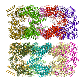
Then, the alignment of the strcture to every region can be accomplished by selecting Align to... ->Each selected region. This aligns the structure (and its simulated density map) to each of the regions that are selected, or ALL regions if none are selected. Since each region in this segmentation corresponds to a single protein, the structure is aligned successfuly to each one, reproducing the strcture of the entire complex, as shown below.
2.1 Getting and segmenting the density map
As another example, we will use the density map of bacteriophage lambda at 14.5Å resolution, which can be downloaded from this link. This map was segmented at a threshold of 3.5, and only 1 smoothing step of size 10.0Å was taken. Because this map is very large, taking more steps typically results in memory problems on 32-bit systems. After this grouping step, a total of 394 regions result. The density map and the segmented regions are shown below.
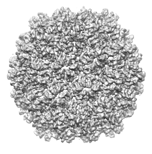
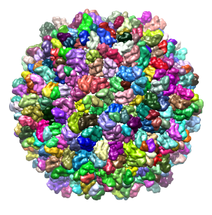
Note: Rendering many small surfaces can be time-intensive, and anything over a few thousand surfaces can make Chimera slow down considerably. Hence, Segger only displays up to 2000 surfaces. In this example, in the intial segmentation, you will not see the entire map covered with regions, because only the first 2000 are actually displayed. The only way to see a more complete segmentation is to group the regions, bringing their number down, after which all of them are displayed.
2.2 Choosing regions to keep
The regions that make up an asymmetric unit (ASU) can be seen in this segmentation, and can be selected together within the Chimera window - use Ctrl+Click for the first region and Shift+Ctrl+Click for all subsequent regions. Then, to keep only these regions, choose Regions->Invert selection, and then Regions->Delete selected. The remaining regions are shown in the image below.
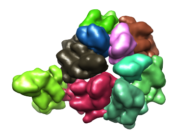
As can be seen above, there are 10 regions, however an ASU actually contains only 7 proteins. Thus, for some of the proteins, two regions correspond to each protein. If we tried to smooth further, to attempt to obtain a single region for each protein, regions from different proteins merge first. So for this map, when smoothing, a point can't be reached in which each region corresponds to a protein. This leads to having to deal with over-smoothing and/or multiple regions per protein.
2.3 Dealing with over-smoothing and multiple regions per protein
The smoothing and grouping process would ideally be stopped just before regions corresponding to different proteins or molecular components merge. This can only be done by visual inspection of the regions after grouping.
The grouping process can be easily undone, by selecting Regions->Ungroup ALL to ungroup all regions, or selecting the region(s) to ungroup and then selecting Regions->Ungroup selected. This can be done repeatedly until all regions are from single proteins. When each protein consists of multiple regions, to get regions corresponding to single proteins, the regions that belong to the same protein can then be selected, and joined by selecting Regions->Group selected.
2.4 Aligning a structure to regions - user selection
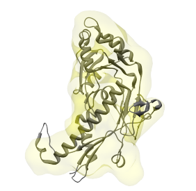
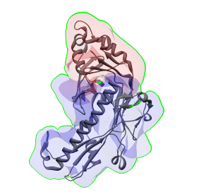
In this example, we can align a protein structure to single and multiple regions. A structure that fits well into this map is PDB:3BQW. It should be centered, and have a density map generated, as before. Then select either a single region to align it to, and choose Align to...->Selected region, or select two regions that appear to correspond to the same protein, and choose Align to...->Combined selected regions. If the right regions are selected, the alignments will look like in the images below. In the image on the left, the structure was aligned to a single region (using Align to...->Selected region), and in the image on the right, structure was aligned to two selected regions (using Align to...->Combined selected regions).
Instead of relying on the user to select the correct regions for alignment, Segger can automatically generate candidate groups of regions to align the structure to. After aligning the structure to each of the generated groups, the alignment with the highest cross-correlation is kept. Groups can be generated in two ways:
2.5 Aligning a structure to regions - automatic grouping starting with one region
In the first way, the user selects a single region, and groups are generated around this region. To use this approach, select any of the regions in the segmentation above, and choose Align to...->Regions around selected. After trying several potential groups, all of which include the region selected, the group of regions that produces the correct alignment is found (even if this group actually only contains 1 region). In the map above, selecting any of the regions, less than ~5 groups are actually generated, and hence the alignment process is still extremely fast.
2.6 Aligning a structure to regions - automatic grouping of all regions
In the second approach, groups of regions generated from all the segmented regions. For this mode, choose Align to...->Groups of regions. Groups are generated in combinatorial fashion, however all groups have only adjacent regions (i.e. in every group, every region is adjacent to at least one other region). The latter condition helps to keep the number of groups down dramatically.
The groups are also filtered such that they don't have a volume that is too different than that of the structure (computed from the density map of the structure at the currently selected threshold), and they don't have a bounding radius that is very different than that of the structure. This filtering also helps to decrease the number of groups considered, without eliminating groups that will lead to the correct fit.
Note: When working with a lot of regions, this process can result in very many groups, and the alignment process can take a long time.
In this example, only 22 groups are generated, and the structure is aligned to each of these groups, with the method selected in the Align to... drop down menu (principal axis transform or rotational search - both methods will work in this case, but the first one is faster).
During the alignment process, a file is created which contains all the cross-correlations scores, sorted in decreasing order. This file may show less than 22 fits, since only the fits with unique transforms are kept (different alignments can result in the same final transform for the fitted structure). The file in the same folder as the density map, emd_1507.mrc, and is named emd_1507_fits_sorted.txt. The first 10 entries in the file are:
2 - structure: 3BQW.pdb, cross-correlation: 0.458
3 - structure: 3BQW.pdb, cross-correlation: 0.450
4 - structure: 3BQW.pdb, cross-correlation: 0.447
5 - structure: 3BQW.pdb, cross-correlation: 0.446
6 - structure: 3BQW.pdb, cross-correlation: 0.420
7 - structure: 3BQW.pdb, cross-correlation: 0.409
8 - structure: 3BQW.pdb, cross-correlation: 0.185
9 - structure: 3BQW.pdb, cross-correlation: 0.166
10 - structure: 3BQW.pdb, cross-correlation: 0.163
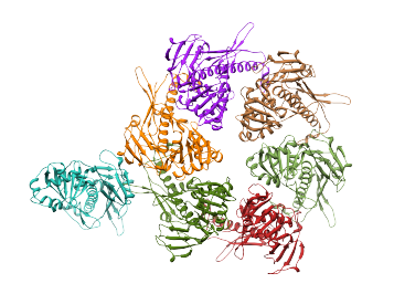
The top 7 cross-correlation scores are much higher than the rest. This indicates that there are 7 good alignments for the structure. In fact, the top 7 alignments produced the correct fits for the protein structure which recreate the entire ASU. To generate the structure of the complete ASU, enter '7' in the field to the right of "top # of fits to place", and press the Place button. This places the structure in the alignments with the top 7 cross-correlation scores, making a copy of the structure in each alignment, and also saving a .pdb file for each alignment. The results are shown in the image below.
Please contact Greg Pintilie by email with comments and suggestions.


 Home
Home